


The dataset can considered and downloaded from right here.
Steps to observe
To carry out an Exploratory Information Evaluation (EDA) on the dataset, we are going to observe these predominant steps:
1. Information Inspection
2. Information Cleansing
3. Information Visualisation
4. Speculation Testing
Step 1: Information Inspection
Information inspection is step one in any evaluation, whether or not the aim is to construct fashions or carry out an EDA, as in our case.
The intention is to look at totally different elements of the info to determine any points that want consideration in the course of the cleansing course of.
Consider it as a check-up completed by medical doctors earlier than making a analysis or prescription.
Importing Obligatory Libraries
For this evaluation, we’ll primarily use `pandas` for knowledge manipulation, `numpy` for numerical operations, and `matplotlib` together with `seaborn` for knowledge visualisation.
Loading the Information
Utilizing the pandas library, you’ll be able to simply load knowledge with features like read_csv, read_excel, and so forth., relying on the file format. Since our dataset is in CSV format, we’ll use the read_csv operate to load it.
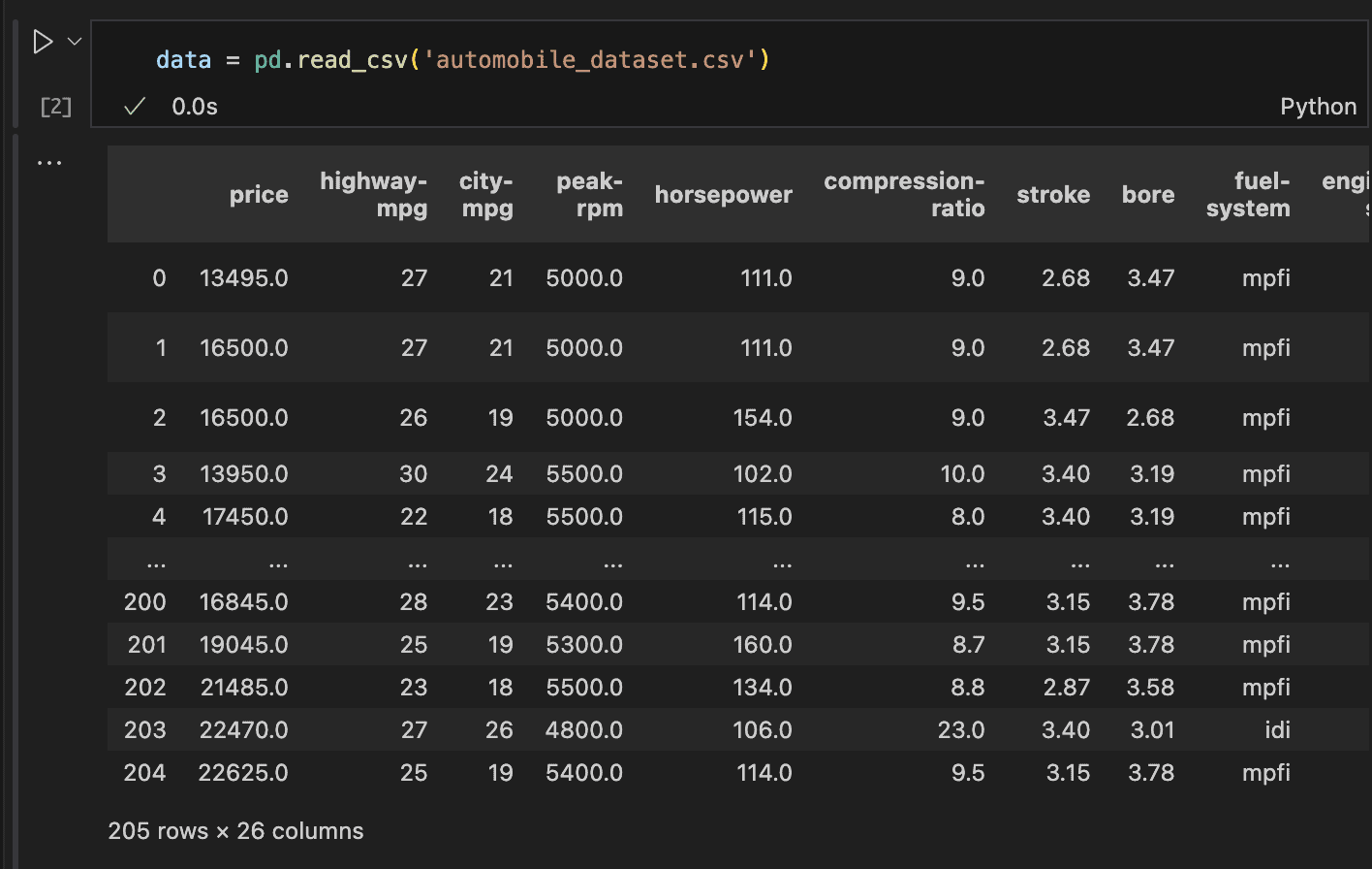
Within the code above, we may see the variety of rows and columns, however there’s extra we have to examine.
What number of columns have lacking values? How can we view all 26 columns and perceive what they signify?
Accessing the columns
To get a complete overview of the dataset, together with particulars like the info sorts, variety of non-null entries, and column names, we are able to use the information() methodology in pandas.
This methodology gives all the things we have to know in regards to the dataset at a look.
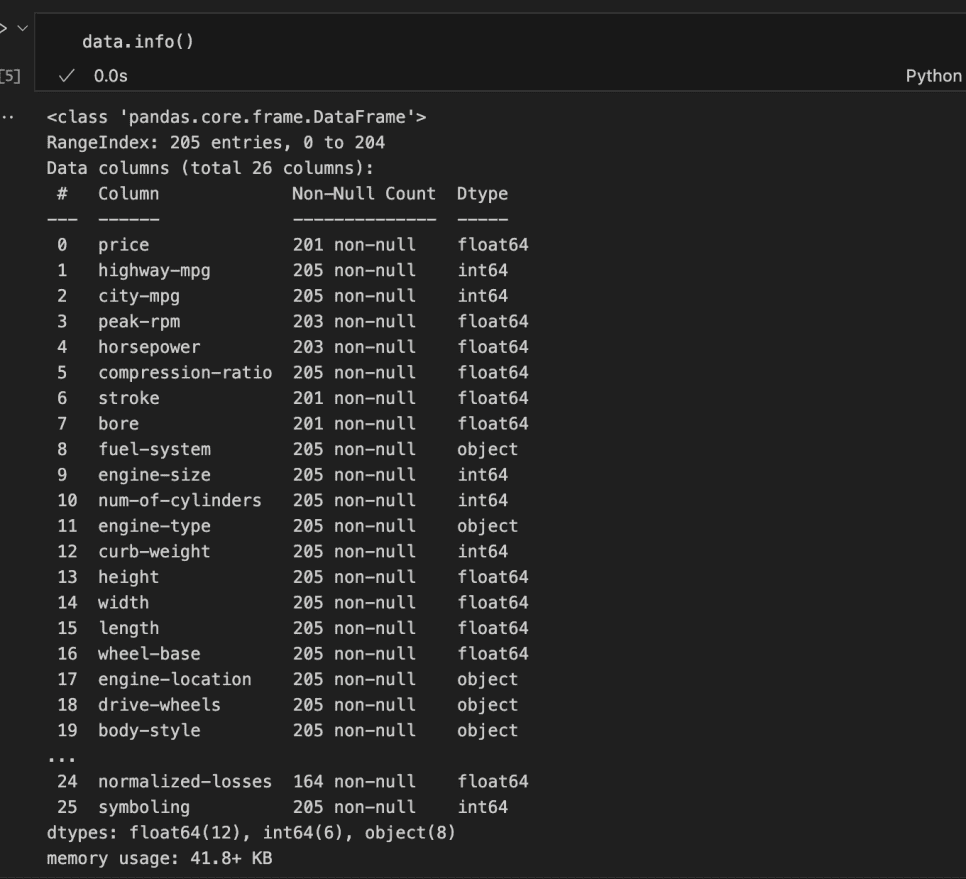
Within the code above, we may partially entry the dataset’s options. Nevertheless, not all columns have been listed.
From these displayed, we are able to determine columns with lacking values, the info forms of every column, and the reminiscence utilization.
It may be noticed that 12 columns are of float knowledge sort, 6 are integers, and eight are strings/objects. Which means 18 columns are numerical, whereas 8 are categorical or ordinal.
Coping with Null values
Coping with null values is important and can’t be averted. For instance, out of the 205 complete rows, the value column has solely 201 non-null entries, horsepower and peak-rpm have 203, and stroke and bore have 201, amongst others.
To get a clearer image, we are able to use the isna() methodology adopted by sum() to return the variety of null values in every column.
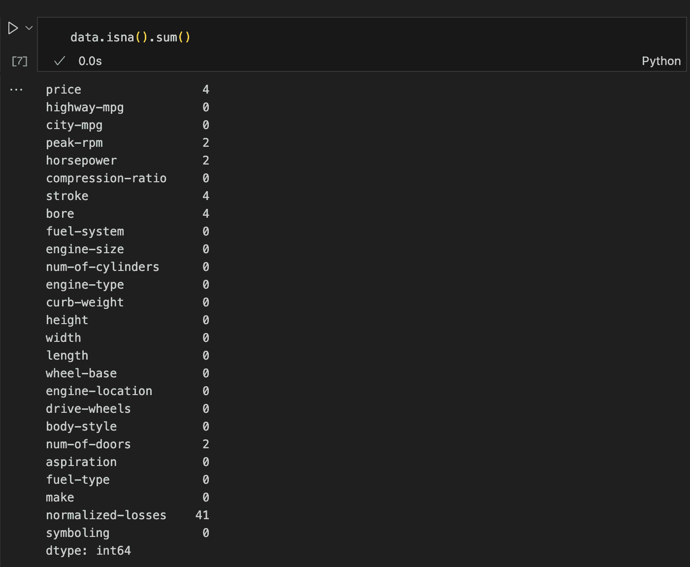
This methodology reveals all the things we have to find out about lacking values, displaying that we have to deal with seven columns in complete.
Duplicate Rows
One other vital side to examine is the presence of duplicate rows. Fortunately, Pandas makes this course of easy.
By utilizing the duplicated() methodology adopted by sum(), we are able to rapidly decide the overall variety of duplicate rows within the dataset.
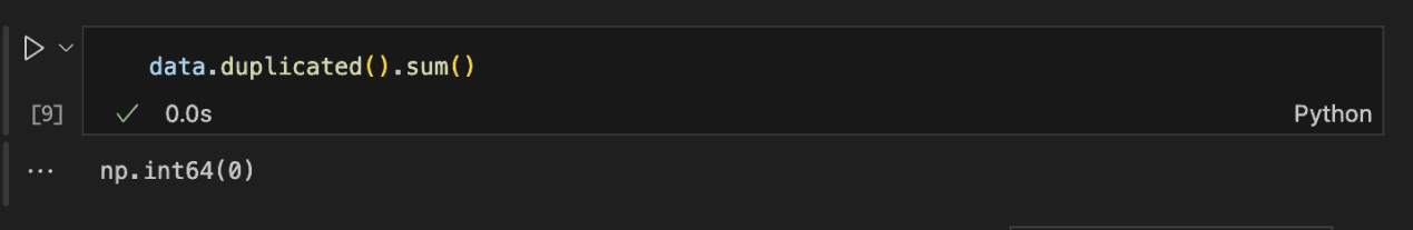
For the reason that return worth is 0, we are able to confidently say that there are not any duplicate rows within the dataset.
Statistical Illustration of Information
To hold out this evaluation, the describe() methodology in Pandas gives a simple solution to view key statistical values for all numeric options. See the code and outcome under for an instance.
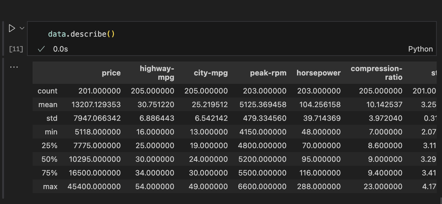
Details about the rely, imply, customary deviation, min, 25-percentile, 50-percentile (median), 75-percentile, and most worth for every column will be simply accessed.
This info reveals that almost all options may need distributions near regular and therefore has no outliers. That may be verified utilizing an histogram and field plot.
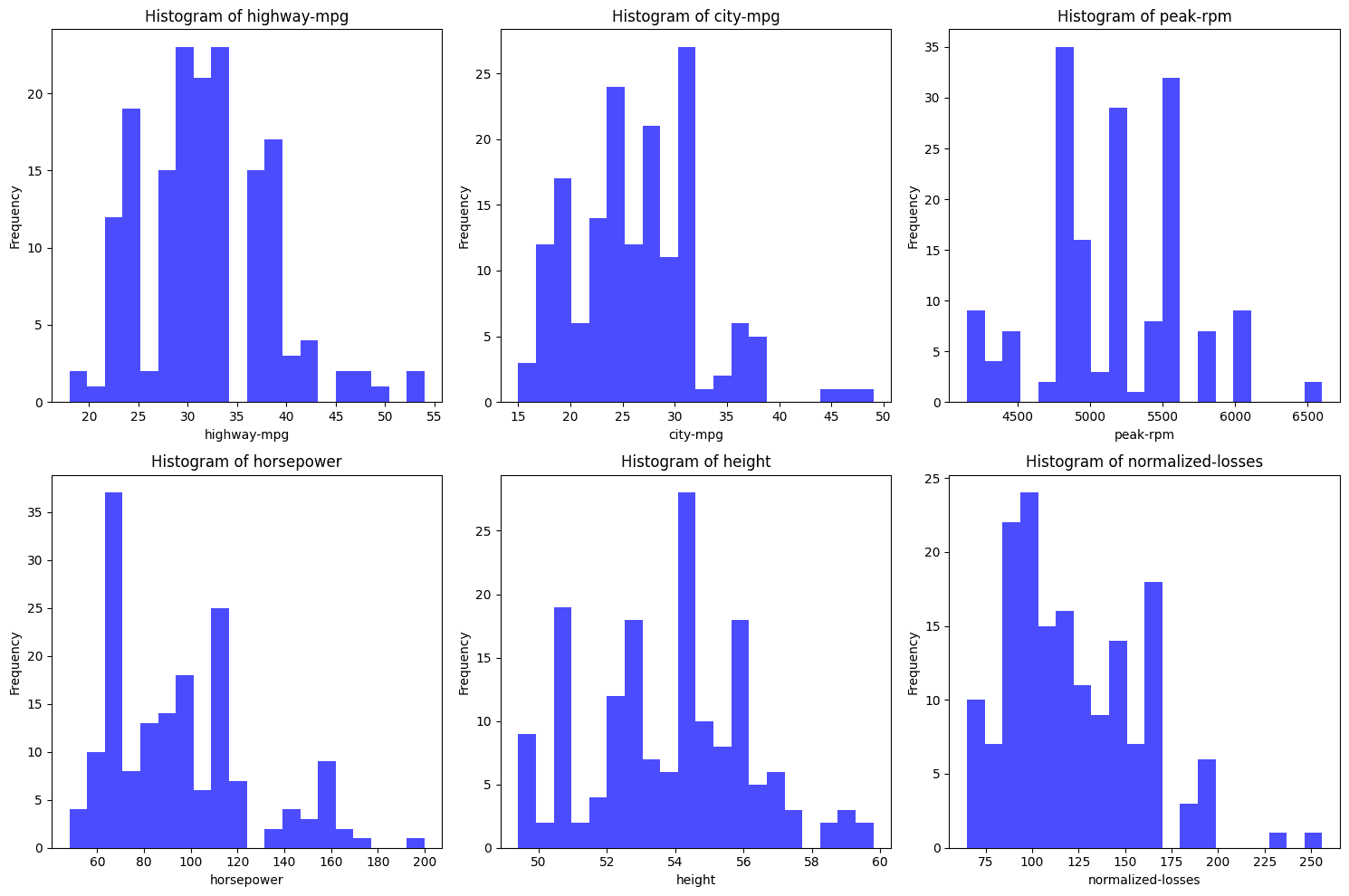
From the histograms above, none of them appear to completely observe a standard distribution. Right here’s a fast evaluation of every:
- highway-mpg: This distribution seems bimodal (two peaks) somewhat than usually distributed which is bell formed. The bimodality suggests two distinct group which might be a gaggle of quick automobiles and fewer quick automobiles.
- city-mpg: Just like highway-mpg, this distribution isn’t usually distributed. It additionally seems bimodal with two peaks.
- peak-rpm: This histogram is kind of irregular with a couple of distinguished peaks, suggesting that the info is skewed and never usually distributed.
- horsepower: The distribution is skewed to the proper, that means there are extra knowledge factors with decrease horsepower, and the tail extends in direction of increased horsepower values. This isn’t a standard distribution.
- top: The peak histogram is the closest to a standard distribution. It isn’t completely regular however it’s fairly shut.
- normalized-losses: This distribution reveals a proper skew, the place most knowledge factors are focused on the decrease aspect and an extended tail stretches in direction of increased values. That is additionally not usually distributed.
Regular distribution have numerous traits which incorporates equal imply and median, a bell formed distribution which additionally means they’re symmentric and subsequently has no skew and eventually, no outliers.
It’s a good method to confirm totally.
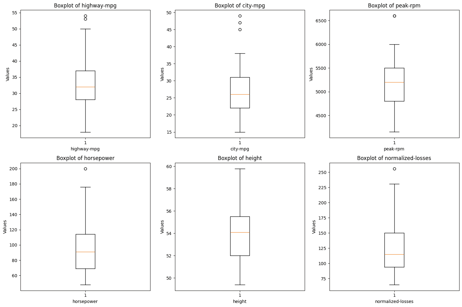
The boxplots above reveals that a number of the variables include outliers. The factors exterior of the whiskers of the plots are outliers and despite the fact that they don’t seem to be many, they have to be handled.
From the perusing step, we all know we have now to take care of lacking knowledge, and outliers.
Step 2: Cleansing the info
Information cleansing includes getting ready the info in a method that makes it appropriate for evaluation.
Sorting Out Lacking Rows
From the earlier step, we all know there are lacking values within the value, num-of-doors, peak-rpm, horsepower, stroke, bore, and normalized-losses columns.
Whereas we are able to exchange these with the imply or median primarily based on statistical reasoning, it’s vital to additionally contemplate the context.
For example, if a characteristic is particular to a sure producer, it could be extra applicable to fill in lacking values with what’s frequent for that producer.
First, let’s assess the rows with lacking horsepower values to determine the most effective method for filling them in.
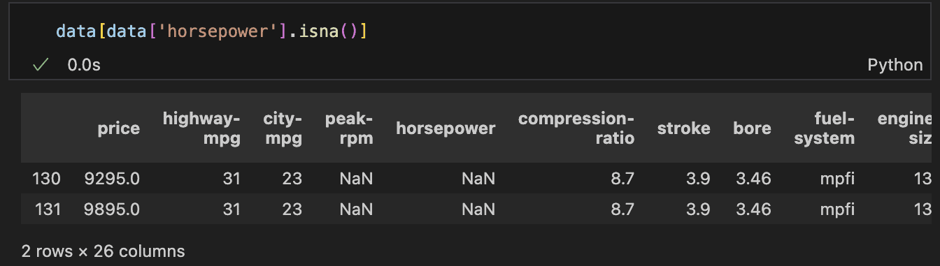
– Horsepower and peak-rpm
There are two rows the place each horsepower and peak-rpm are lacking. A better look reveals that these rows belong to the identical automotive model, and notably, these are the one two information for that producer within the dataset.
This means that there are not any historic values to reference, making it inappropriate to easily use the common or median of your complete column.
It is because a automotive’s horsepower is influenced by numerous elements, together with the producer.
In a real-world situation, with inadequate knowledge and an incapacity to afford dropping extra rows, the best choice can be to analysis the automotive model.
The dataset incorporates particulars just like the variety of doorways and the physique fashion (e.g., wagon or hatchback), which may assist determine the particular mannequin or an analogous one to estimate the lacking horsepower.
Nevertheless, on this case, we are going to drop these rows. As well as, it’s value noting that the normalised-losses—which signify the historic losses incurred by an insurance coverage firm for a particular automotive, after being normalised—are additionally lacking.
Since normalised losses are essential on this evaluation, we are going to exclude rows with out this knowledge. If this have been a modeling downside, we’d contemplate coaching a mannequin to foretell these losses, after which use the mannequin to estimate the lacking values.
– Stroke and bore options
Subsequent, let’s talk about the stroke and bore options. The bore refers back to the diameter of the engine’s cylinders, measured in inches. Bigger bores permit for bigger valves and elevated airflow.
The stroke, then again, is the space the piston travels contained in the cylinder, additionally measured in inches. Longer strokes usually present extra torque.
There could also be a correlation between these options and the normalised losses, making them probably vital.
Upon inspecting the rows with lacking stroke and bore, we discover that 4 rows are lacking each options.
These rows correspond to automobiles from the Mazda model. We should always look into historic information for Mazda to find out the standard values for stroke and bore of their autos.
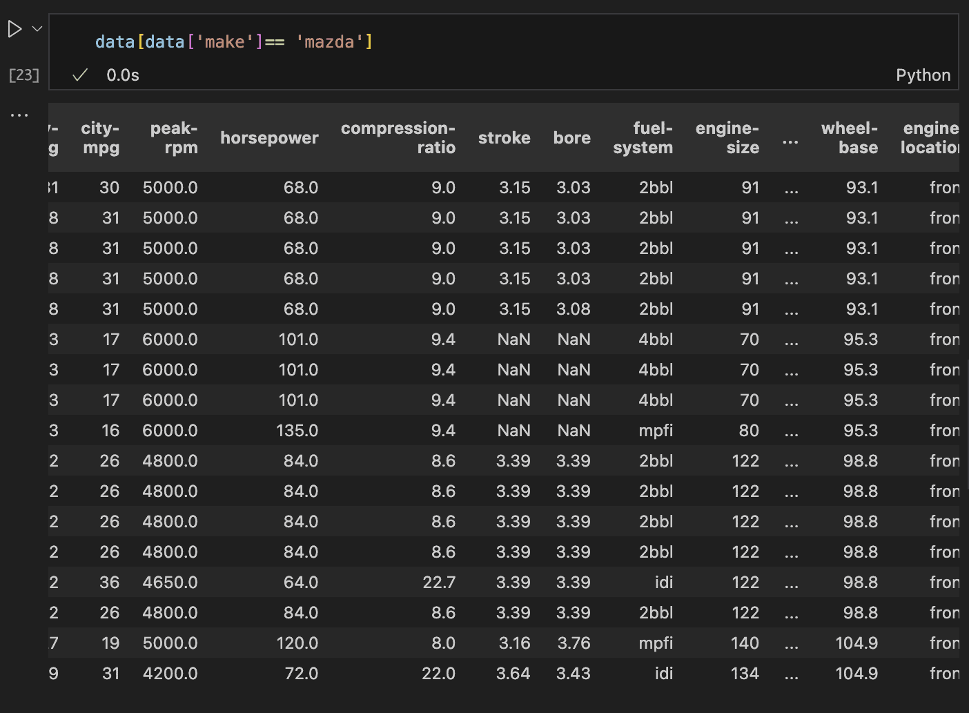
The code and outcome above confirms that historic knowledge is accessible. Whereas the most effective method can be to conduct analysis, a viable different is to switch the lacking values with the common values from related information.
This ensures the alternative values keep inside a sensible vary. To proceed, we first calculate the common stroke and bore values for Mazda autos within the dataset.
As soon as we have now these averages, we are able to exchange the lacking values accordingly. This may be completed by grouping the info by the automotive producer after which computing the common for the stroke and bore columns.
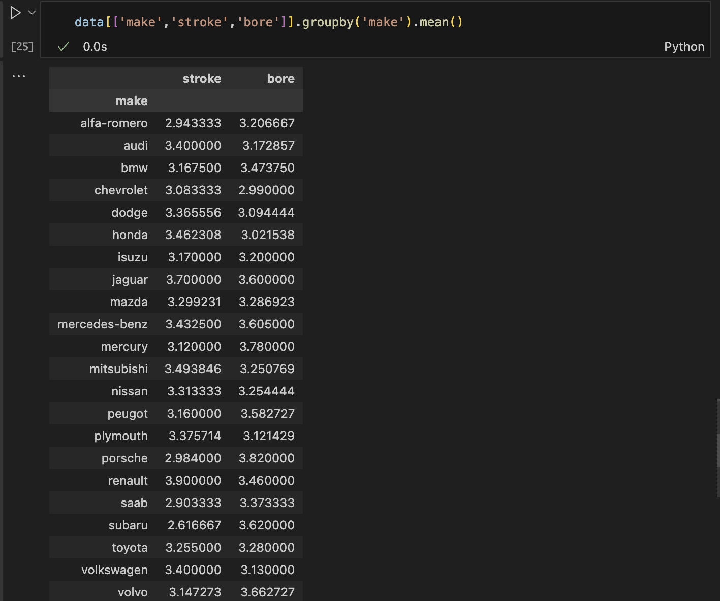
The imply values for Mazda’s stroke and bore are roughly 3.3, rounded to the closest decimal.
We will exchange the lacking values (NaN) with these averages. We will apply the identical technique for the lacking costs.
First, we determine the rows with lacking costs, examine the automotive manufacturers, after which determine the most effective plan of action.
There are three totally different automotive manufacturers with lacking costs, which even have their normalised losses lacking. Since our evaluation focuses on normalised losses, we’ll drop rows with lacking normalised losses for this evaluation.
Dealing with outliers
Concerning outliers, there are numerous approaches to dealing with them relying on the dataset’s meant use. When constructing fashions, one possibility is to make use of algorithms which might be strong to outliers.
If the outliers are as a result of errors, they are often changed with the imply or eliminated altogether.
On this case, nonetheless, we are going to depart them as they’re. This determination is predicated on their shortage throughout variables, which permits us to retain all cases within the knowledge.
The outliers are usually not faulty; in reality, having extra knowledge would allow us to seize a broader vary of their cases.
With that determined, let’s proceed with the info cleansing:
- First, take away all rows with lacking normalised losses. This may also deal with rows with lacking costs and horsepower.
- Then, fill within the imply stroke and bore values for Mazda solely.
- Lastly, print the sum of all remaining null values to substantiate the cleansing course of.
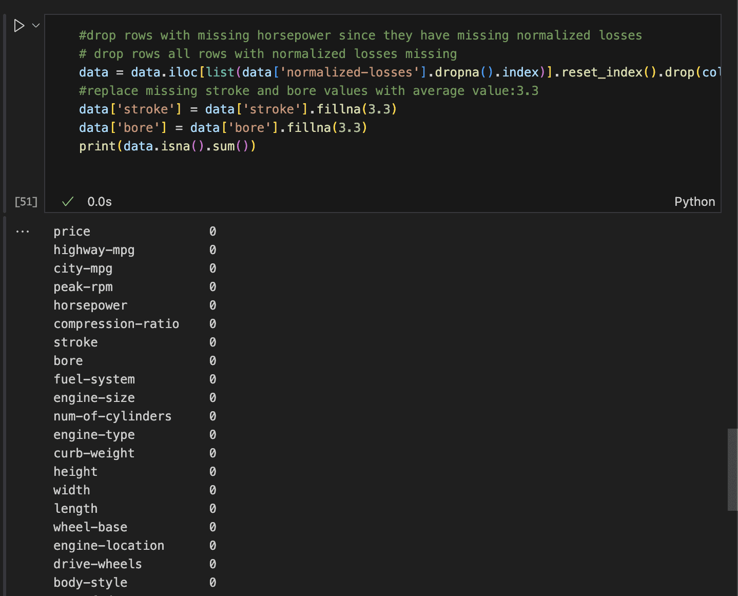
This leaves us with zero lacking values in every row.
Drop Pointless Columns
At this level, it’s essential to be clear in regards to the focus of the evaluation and take away irrelevant columns.
On this case, the evaluation is centered on understanding the options that affect normalised losses.
With a complete of 26 columns, we must always drop these which might be unlikely to contribute to accidents or injury.
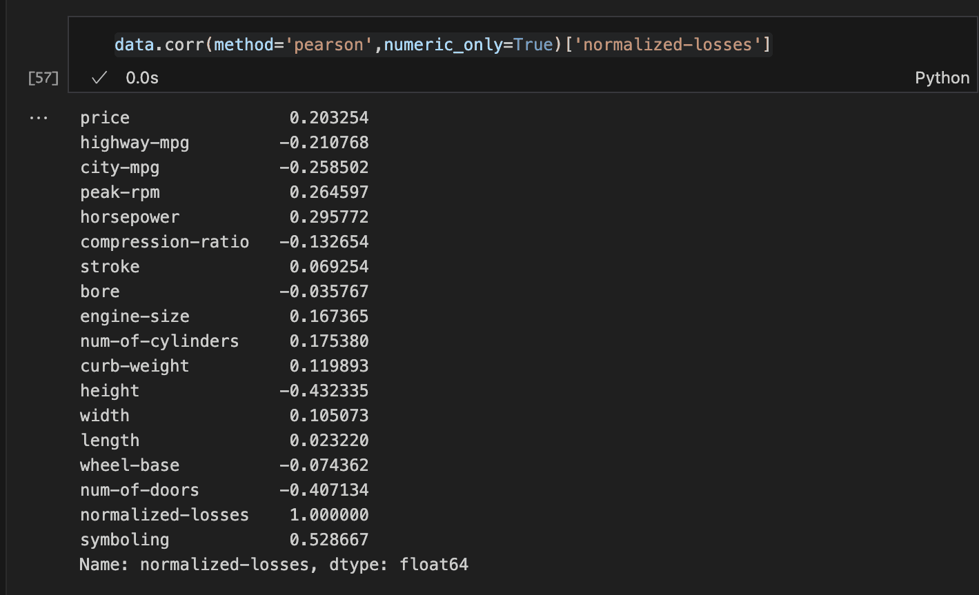
An easy method is to look at the correlation of the numeric options with normalised losses. This may be simply completed utilizing the Corr methodology.
Step 3: Visualising the info
To successfully carry out knowledge visualisation, we are able to formulate key questions that want solutions:
Some examples will be:
- Does a sure physique sort,gas sort or aspiration result in elevated insurance coverage loss?
- What’s the relationship between chosen options and normalised losses?
To reply the query about physique sort, we are able to analyze the connection between physique sort and normalised losses. Right here’s how:
- Choose the body-type and normalised losses columns.
- Group the info by body-type and calculate the imply normalized losses for every group.
- Use Seaborn’s barplot to visualise the imply normalised losses by physique sort.
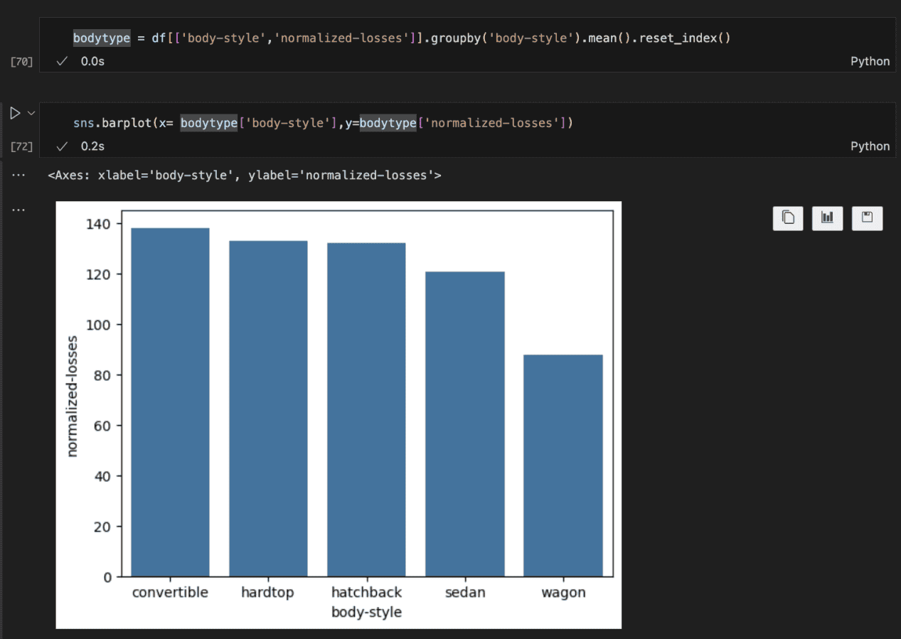
The plot above reveals that imply losses certainly differ primarily based on physique sort. Convertibles have the very best common quantity paid for losses by insurance coverage firms, whereas wagons have the bottom.
I think it is because of the truth that convertibles are typically sport automobiles and as such constructed for velocity. This could result in extra accidents and extra causes to increased insurance coverage pay.
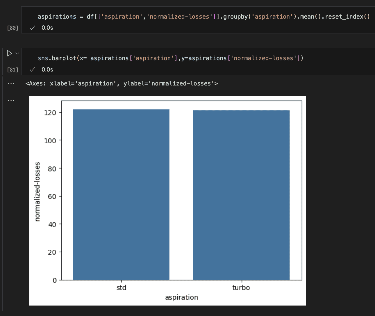
The image above reveals whether or not or not a automotive is customary (naturally supercharged) or as turbo has no impact on the losses. I discover this stunning.
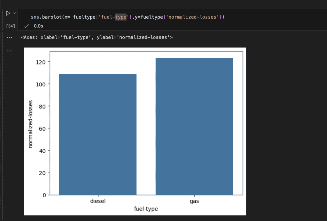
Checking the gas sort reveals that automobiles operating on gasoline incur extra losses for insurance coverage firms than diesel-powered autos.
This might be as a result of gas-powered automobiles usually present higher acceleration, main drivers to push them tougher and probably rising the probability of accidents.
The subsequent type of evaluation is to examine the connection between numerical options.
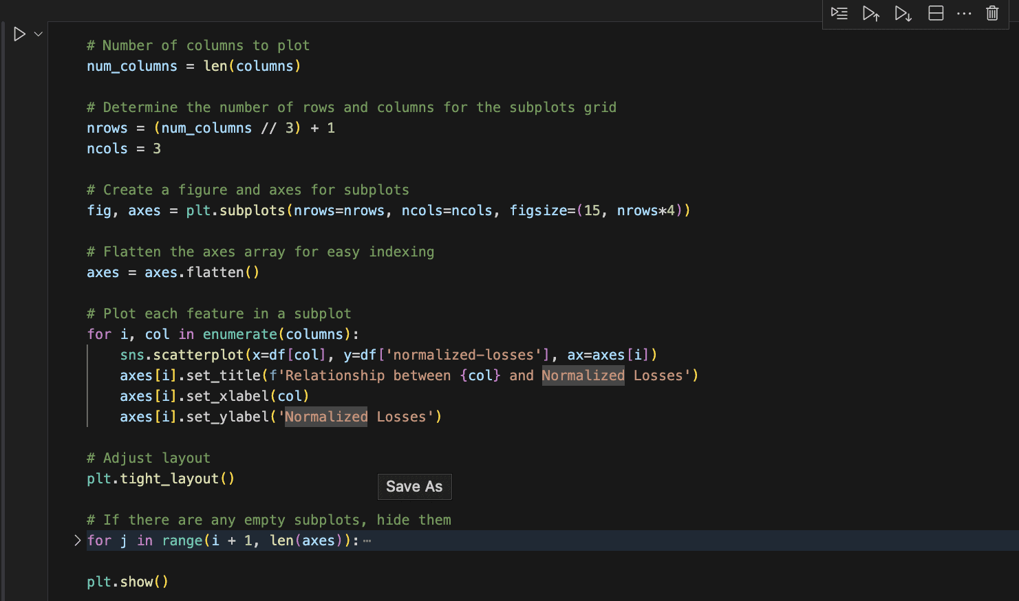
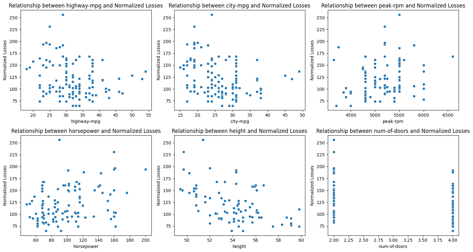
The subplots under present the connection between chosen options and normalised losses.
Key Takeaways:
- Gasoline Effectivity: There’s a slight constructive correlation between a automotive’s gas effectivity in each metropolis and freeway driving and the normalised losses.
- Engine Efficiency: The engine velocity at which most horsepower is produced (peak RPM) reveals a slight constructive correlation with normalised losses. As well as, there’s a good stronger constructive relationship between horsepower and losses. Increased horsepower usually results in quicker acceleration and better prime speeds, which might improve the probability of accidents and, consequently, extra injury.
- Automotive Peak: Taller automobiles are inclined to incur fewer losses. That is an instance of unfavourable correlation. It could be as a result of higher visibility and enhanced crash safety supplied by their taller roofs, significantly in sure forms of collisions.
- Variety of Doorways: There’s a reasonable constructive correlation between the variety of doorways and normalized losses, with automobiles having fewer doorways (sometimes two-door automobiles) incurring extra losses. This might be as a result of many two-door automobiles are sports activities automobiles, which are sometimes pushed extra aggressively.
Step 4: Speculation Testing
Whereas visualisations can counsel potential constructive relationships, it’s vital to check the statistical significance of those relationships.
Are the options actually correlated, or is it simply as a result of likelihood?
When performing significance checks, a number of elements have to be thought of. These embody the kind of knowledge (e.g., numerical vs. categorical, numerical vs. numerical), the normality of the info, and the variances, as many statistical checks depend on particular assumptions.
On this case, we’re evaluating our numerical variables with the normalised losses utilizing Spearman’s Rank Correlation because the knowledge distribution isn’t regular.
Let’s outline our hypotheses:
Null Speculation (H₀): There is no such thing as a correlation between the 2 variables.
Various Speculation (H₁): There’s a correlation between the 2 variables.
We set the importance stage (alpha) at 0.05. If the p-value is lower than alpha, we reject the null speculation and conclude that there’s a important relationship.
Nevertheless, if the p-value is larger than alpha, we fail to reject the null speculation, that means no important correlation is discovered.
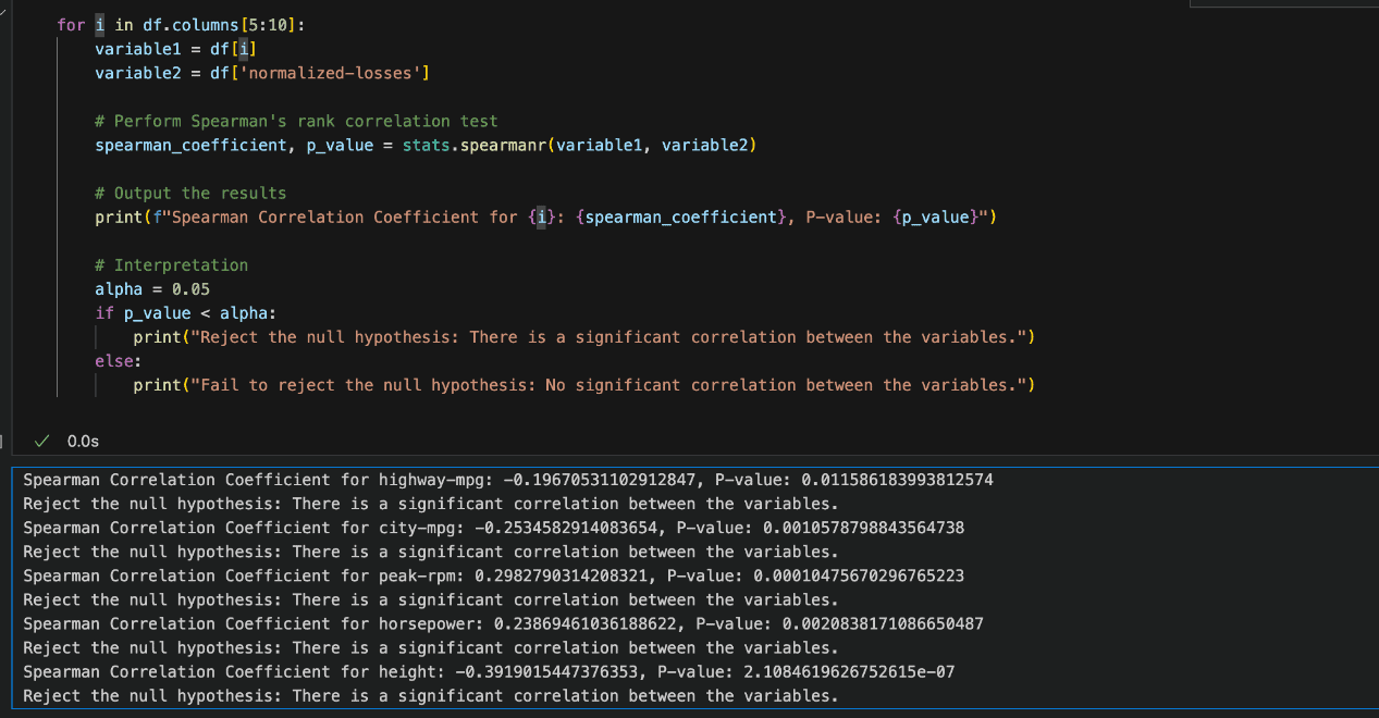
Primarily based on the picture above, the outcomes point out that our assumptions are statistically important, and for every variable, the null speculation is rejected.
Conclusion
From the evaluation, it’s evident that sure elements associated to a automotive’s stability and acceleration capabilities usually result in elevated insurance coverage losses.
This complete evaluation coated numerous approaches to knowledge wrangling and visualisation, uncovering useful insights.
These findings can help insurance coverage firms in making extra knowledgeable selections, predicting potential losses related to particular automotive fashions, and adjusting their pricing methods accordingly.


